---
title: "Sentiment Analysis of NYC's Mayor Eric Adams' Speeches"
subtitle: "Problem-Solving in Action"
author: "Arcenis Rojas"
date: "04/03/2024"
editor: visual
execute:
warning: false
error: false
bibliography: eric-adams-speeches.bib
categories:
- Web Scraping
- Text Analysis
- Animation
---
## Project description
This project came from a question that I had about how the sentiment in NYC Mayor Eric Adams' speeches might have changed over the last few years given some of the different challenges he's had in office ranging from COVID-19-related policies to more recent issues with immigration in NYC. As often happens, this simple question introduced unanticipated challenges and again made me really grateful to the open-source community.
For this analysis I relied heavily on [tidyverse](https://www.tidyverse.org/) [@tidyverse] packages for data wrangling; the [rvest](https://rvest.tidyverse.org/) [@rvest] and [polite](https://dmi3kno.github.io/polite/) [@polite] packages for webscraping; the [tidytext](https://juliasilge.github.io/tidytext/) [@tidytext], [textdata](https://github.com/EmilHvitfeldt/textdata) [@textdata], and [textclean](https://github.com/trinker/textclean) [@textclean] packages for text analysis functions; and the [ggplot2](https://ggplot2.tidyverse.org/) [@ggplot2], [ggwordcloud](https://lepennec.github.io/ggwordcloud/index.html) [@ggwordcloud], and [gganimate](https://gganimate.com/) [@gganimate] packages for visualization.
## Getting speech data
To perform this analysis I would have to find a repository of his speeches online and figure out how to scrape them. Because I thought there would be a lot of speeches, I knew that I would run into issues dealing with having to add delays to my scraping function so as not to run into conflict with the rules of the site. I also thought about the problem of having to scrape pages with Javascript on them and remembered that [Hadley Wickham](https://hadley.nz/) [posted on LinkedIn](https://www.linkedin.com/feed/update/urn:li:activity:7159172919758065665?updateEntityUrn=urn%3Ali%3Afs_feedUpdate%3A%28V2%2Curn%3Ali%3Aactivity%3A7159172919758065665%29) about an experimental update to [rvest](https://rvest.tidyverse.org/) that included tools for scraping live sites using [chromote](https://rstudio.github.io/chromote/). Without remembering this I probably would not have pursued the project because the alternative for scraping live web pages with R is [RSelenium](https://docs.ropensci.org/RSelenium/articles/basics.html) (at least as far as I know), which requires a lot more set-up work than this project would have been worth.
As far as dealing with the robots on the NYC news site, I also wanted to scrape in an ethical way. Thinking about this led me to two things: 1) [Rules for ethical webscraping](https://towardsdatascience.com/ethics-in-web-scraping-b96b18136f01) and 2) the [polite](https://dmi3kno.github.io/polite/) package. First, there is the practical consideration that some sites place limits on the frequency with which they will serve results to clients and if the scraping process doesn't respect that one may end up getting one result with content and a bunch of empty results thereafter if not just outright errors. Aside from this practical consideration, my position is that if I'm getting all this great data for free (that someone is paying to host) the least I can do is identify myself to the host so the host knows I mean no harm.
### Finding speech transcripts
Once I decided to go ahead, the first challenge was to get transcripts of Mayor Adams' speeches. A simple web search led me to the [NYC.gov](https://www.nyc.gov/) website which has a section for [news coming out of the office of the Mayor](https://www.nyc.gov/office-of-the-mayor/news.page). I noticed that this site had more than his speeches, but there were some titles of articles that started with the word "Transcript". After looking through a few pages I saw that this was the case for many articles, so I thought I could use this to isolate the articles that contained speeches. The next step was figuring out how to scrape the data.
### Challenges in webscraping
I first figured out that I would have to scrape in two stages. In the first stage, I would have to scrape all of the pages containing news article titles and their corresponding links, which would require knowing how many pages of links there are. I would then have to filter these links for the ones that contained speech transcripts. In the second stage I would have to go to each of the links from the first stage and scrape the speech text.
Going into the first stage I wanted to use `polite::nod()` to jump from one page to the next. However, I learned that all of the pages with search results were live pages (Javascript) and `polite::scrape()` is designed to work with static elements, so there were elements of the page that I wasn't getting. I thought I would either be stuck or have to make a trade-off between getting output and behaving ethically until I found [yusuzech's Cheat Sheet for Web Scraping Using R](https://github.com/yusuzech/r-web-scraping-cheat-sheet) in which he talks about different ways to deal with this particular challenge. There I learned about an [entry in Hartley Brody's blog](https://blog.hartleybrody.com/web-scraping-cheat-sheet/) containing his Web Scraping Cheat Sheet. In the "More Advanced Topics" section he mentioned that a page with live elements (Javascript) requires that the content be in static form *somewhere* on the server. I was able to find that page for the NYC site, which then required identifying the links that I needed using [regex](https://en.wikipedia.org/wiki/Regular_expression), which was a much smaller problem than choosing between getting data from a live site and scraping ethically.
### Webscraping code
```{r}
#| label: webscraping-load-packages
library(tidyverse)
library(xml2)
library(rvest)
library(polite)
library(tidytext)
library(textclean)
library(textdata)
library(ggwordcloud)
library(gganimate)

# Resolve common namespace conflicts about function names
conflicted::conflict_prefer("filter", "dplyr")
conflicted::conflict_prefer("lag", "dplyr")
if ("tidymodels" %in% .packages()) tidymodels_prefer()
```
Below is the code that I used for scraping the data. I tried to parallize this code, but I learned that code that uses external pointers will error out with the different packages I tried for parallelization.
Here I declare a function for the first stage of the web scraping process which takes as arguments the `polite::bow()` object and the number of the search page to scrape.
::: callout-note
This function jumps to the static site that lists the search results in `polite::nod()`. The query in the path string shows that all of the results are from the dates between 12/31/2021 and 12/31/2024.
:::
```{r}
#| label: webscraping-get-article-links-fun
#| code-fold: show
#| eval: false
get_article_links <- function(bow_obj, srch_pg_num) {
message(str_c("Scraping links from page ", srch_pg_num))
search_sess <- nod( # <1>
bow_obj,
path = str_c(
"/home/lscs/NewsFilterService.page",
"?category=all&contentType=all&startDate=12/31/2021&endDate=12/31/2024&",
"language=english&pageNumber=",
srch_pg_num
)
)
scrape(search_sess) |> # <2>
as_list() |>
pluck("root", 2) |> # <3>
str_extract("\\[\\{(.*)") |> # <4>
str_extract_all('(?<=URL":")[\\/\\-a-z0-9]+') |> # <5>
flatten_chr() |>
str_subset("transcript") |> # <6>
enframe(value = "speech_link") |> # <7>
select(-name)
}
```
1. Jump from the root node of the website to the search page of interest
2. Scrape the HTML as XML text
3. Keep only the second element of the root node (exclude head elements)
4. Keep everything after some additional metadata elements
5. Extract everything that proceeded the text indicating a URL
6. Keep only the URL's that contained the term "transcript"
7. Put the vector of links into a dataframe
The next function scrapes a page containing speech data taking as arguments the `polite::bow()` object, one of the links from the first stage, and a number of the link being read to track progress.
```{r}
#| label: webscraping-get-speech data-fun
#| code-fold: show
#| eval: false
get_speech_data <- function(bow_obj, article_path, speech_num = 1) {
message(str_c("Scraping speech number ", speech_num))
speech_html <- nod(bow_obj, path = article_path) |> # <1>
scrape(accept = "html") |>
html_element(".ls-col .ls-col-body .ls-row.main") |>
html_element(".iw_component .container .col-content")
speech_date <- speech_html |> # <2>
html_elements(".richtext p .date") |>
html_text2()
speech_content <- speech_html |> # <3>
html_element(".richtext") |>
html_elements("p")
data.frame( # <4>
speech_title = speech_html |> # <5>
html_element(".article-title") |>
html_text2(),
speech_date = speech_date,
speaker = speech_content |> # <6>
map(
\(x) {
bold_txt <- x |> html_elements("strong") |> html_text()
ifelse(length(bold_txt) == 0, NA_character_, bold_txt)
}
) |>
flatten_chr(),
speech_text = html_text2(speech_content) # <7>
) |>
filter(
!speech_text %in% speech_date, # <8>
str_detect(speech_text, "^\\#+$", negate = TRUE) # <9>
) |>
mutate( # <10>
speaker = str_extract(speaker, ".*(?<=:)"),
speech_text = if_else(
!is.na(speaker),
str_remove(speech_text, speaker),
speech_text
) |>
str_trim() |>
str_squish(),
speaker = str_remove(speaker, ":$")
) |>
fill(speaker, .direction = "down") |> # <11>
group_by(speech_title, speech_date, speaker) |>
summarise( # <12>
speech_text = str_flatten(speech_text, collapse = " "),
.groups = "drop"
) |>
filter( # <13>
speaker %in% c("Eric Adams") || str_detect(speaker, "Mayor")
)
}
```
1. Jump from the root node of the website to the page containing the speech text and scrape the text
2. Store the date from the text
3. Store all of the content that is in a paragraph element
4. Create a dataframe to organize all the data
5. Create a column for the speech title
6. Extract the bold text which indicates who the speaker is (some transcripts had multiple speakers)
7. Create a column to store the speech text
8. Filter out any rows in which the speech text is the date (the date is stored in a separate column)
9. Remove rows that only contain hash tags in the speech text
10. Clean up the speech text and speaker data columns
11. Fill the speaker column down to ensure that every paragraph has a speaker associated with it
12. Collapse all of the text together by speaker
13. Keep only text spoken by Mayor Eric Adams
Next is the code to actually scrape the data using the above functions. You might notice that I used `possibly()` from the `purrr` package. I used this for error handling because I wanted to be able to filter each of the data sets for any empty results. Of course, empty results were a lot less likely because the `polite::bow()` object stored all the necessary permissions. I thought the redundancy was more helpful than harmful here given how long this code would have to run. This process resulted in 280 search pages and about 1,100 speeches with a couple of seconds of wait time between requests, so I had a strong incentive to minimize errors and to be able to easily identify operations that either returned errors or empty results.
```{r}
#| label: webscraping-code
#| code-fold: show
#| eval: false
# Store the domain of the NYC.gov website
nyc_root <- "https://www.nyc.gov"

# Instantiate a session with permissions to the NYC website
nyc_sess <- bow(nyc_root, user_agent = "arcenis-r", force = TRUE)

# Get the number of pages of news article links
num_search_pages <- read_html_live(
  str_c(nyc_root, "/office-of-the-mayor/news.page")
) |>
  html_element(".main-search-results") |>
  html_text2() |>
  str_extract("\\d+(?= pages)") |>
  as.numeric()

# Get the links to all news articles from each page
speech_links <- tibble(search_page_num = seq(1, num_search_pages)) |>
  mutate(
    page_links = map(
      search_page_num,
      possibly(\(x) get_article_links(nyc_sess, x), NULL)
    )
  )

# Scrape speeches
nyc_mayor_speeches <- speech_links |>
  unnest(page_links) |>
  mutate(speech_number = row_number()) |>
  mutate(
    speech_data = map2(
      speech_link, speech_number,
      possibly(\(x, y) get_speech_data(nyc_sess, x, y), NULL)
    )
  )
```
## Sentiment analysis over time
With the data secured, the next step would be to look at changes in the sentiment of his speeches over time. To do that I tokenized the speech data and used both the AFINN-111 valence lexicon [@nielsen11] and the NRC word-emotion association lexicon [@mohammad13].
```{r}
#| label: load-data
#| echo: false
nyc_mayor_speeches <- read_rds("C:/r-projects/eric-adams-speeches/speech-text-data.rds")
```
```{r}
#| label: clean-speech-data
speech_df <- nyc_mayor_speeches |>
  select(-c(search_page_num, speech_number)) |>
  mutate(
    speech_text = str_to_lower(speech_text) |>
      replace_url() |>
      replace_html() |>
      replace_contraction() |>
      replace_word_elongation() |>
      replace_ordinal() |>
      replace_date() |>
      replace_money() |>
      replace_number() |>
      replace_kern() |>
      replace_curly_quote() |>
      replace_non_ascii() |>
      str_squish() |>
      str_trim(),
    speech_date = mdy(speech_date)
  ) |>
  group_by(speech_date) |>
  mutate(
    speech_id = str_c(
      speech_date |> as.character() |> str_remove_all("-"),
      row_number()
    )
  ) |>
  ungroup()

speech_word_tokens <- speech_df |>
  unnest_tokens(word, speech_text) |>
  anti_join(stop_words, by = "word") |>
  filter(is.na(as.numeric(word)))

speech_tf_idf <- speech_word_tokens |>
  count(speech_id, word, sort = TRUE) |>
  group_by(speech_id) |>
  mutate(speech_word_count = sum(n)) |>
  ungroup() |>
  bind_tf_idf(word, speech_id, n)
```
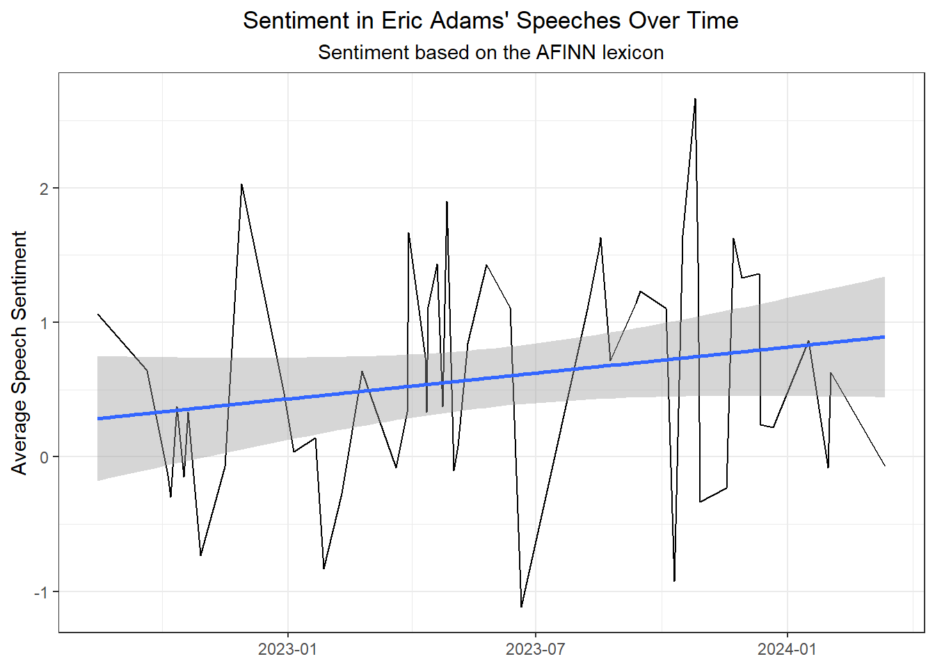
This first plot shows sentiment over time based on the AFINN-111 lexicon with a linear modeling smoother. This lexicon applies a value between -5 (most negative) and 5 (most positive) to each word in the lexicon. I calculated sentiment by date by taking the mean sentiment of all of the words used on each day. It appears that the sentiment in Eric Adams' speeches has become more positive over time.
::: callout-note
I calculated average sentiment by day rather than by speech because Eric Adams made multiple speeches on some days.
:::
```{r}
#| label: plot-sentiment-afinn
speech_word_tokens |>
  inner_join(get_sentiments("afinn"), by = "word") |>
  group_by(speech_date) |>
  summarise(mean_valence = mean(value, na.rm = TRUE), .groups = "drop") |>
  ggplot(aes(speech_date, mean_valence)) +
  geom_line() +
  stat_smooth(method = "lm", formula = y ~ x) +
  labs(
    title = "Sentiment in Eric Adams' Speeches Over Time",
    subtitle = "Sentiment based on the AFINN lexicon",
    y = "Average Speech Sentiment",
    x = NULL
  ) +
  theme_bw() +
  theme(
    plot.title = element_text(hjust = 0.5),
    plot.subtitle = element_text(hjust = 0.5)
  )
```
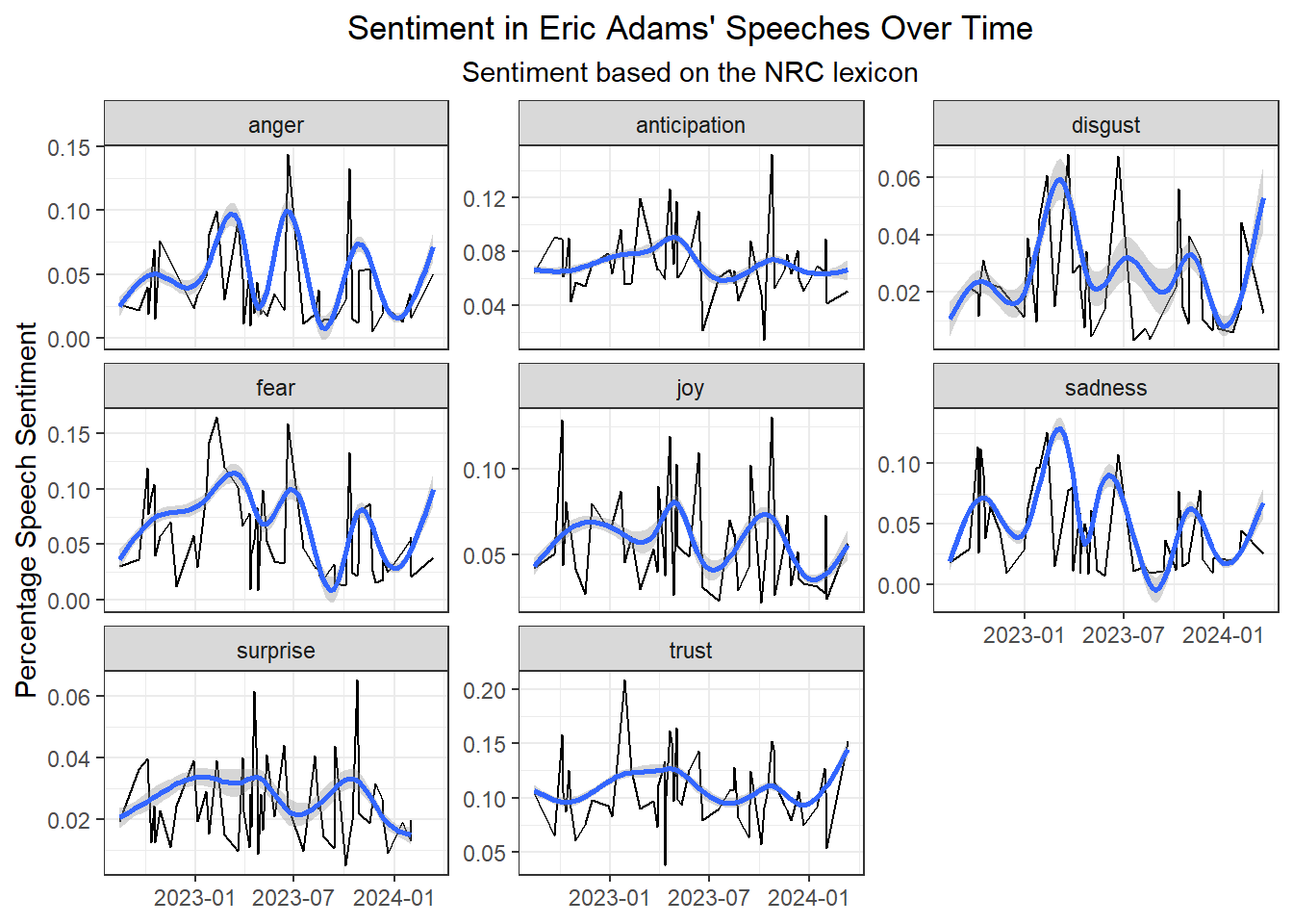
The below plot shows sentiment over time based on the NRC lexicon. This lexicon assigns each word a label indicating a given emotion such as anger, joy, or disgust. It also assigns "positive" and "negative" labels, which I filtered out. For this plot I calculated the percentage of words that were related to each emotion out of all non-stop words in the speech and applied a gamma smoother. This plot shows that there were spikes in disgust, fear, and sadness in the first half of 2023. The reduction of these negative emotions in Eric Adams' speeches could account for the apparent positive trend in the last plot; the emotional content got less negative.
::: callout-note
**Stop words** are words that are inconsequential to determining the meaning of a set of words or distinguish that set of words from other words. They also tend to be very common.
:::
```{r}
#| label: plot-sentiment-nrc
speech_word_tokens |>
  group_by(speech_date) |>
  count(word) |>
  mutate(total_words = sum(n)) |>
  inner_join(
    get_sentiments("nrc") |>
      filter(!sentiment %in% c("positive", "negative")),
    by = "word", relationship = "many-to-many"
  ) |>
  group_by(speech_date, sentiment) |>
  reframe(sentiment_pct = sum(n) / total_words) |>
  ggplot(aes(x = speech_date, y = sentiment_pct)) +
  geom_line() +
  stat_smooth(method = "gam", formula = y ~ s(x, bs = "cs")) +
  labs(
    title = "Sentiment in Eric Adams' Speeches Over Time",
    subtitle = "Sentiment based on the NRC lexicon",
    y = "Percentage Speech Sentiment",
    x = NULL
  ) +
  facet_wrap(~sentiment, scales = "free_y") +
  theme_bw() +
  theme(
    plot.title = element_text(hjust = 0.5),
    plot.subtitle = element_text(hjust = 0.5)
  )
```
## Word cloud animation
Below is a short animation of word clouds for each month in the data. Each word cloud includes 50 words with the highest TF-IDF (term frequency, inverse document frequency) values by month.
```{r}
#| label: word-cloud-animation
#| cache: true
set.seed(98457)
wrdcld_data <- speech_tf_idf |>
  left_join(select(speech_df, speech_id, speech_date), by = "speech_id") |>
  mutate(
    speech_yrmo = floor_date(speech_date, "month")
  ) |>
  group_by(speech_yrmo) |>
  slice_max(tf_idf, n = 50, with_ties = FALSE) |>
  ungroup() |>
  mutate(
    yrmo_label = format(speech_date, format = "%B, %Y") |>
      fct_reorder(speech_yrmo),
    word_size = abs(1 / log(tf_idf)),
    word_color = sample(1:5, n(), replace = TRUE) |> factor(),
    word_angle = 45 * sample(-2:2, n(), replace = TRUE, prob = c(1, 1, 4, 1, 1))
  )

num_frames <- wrdcld_data |>
  distinct(speech_yrmo) |>
  count() |>
  pull(n)

adams_cloud <- wrdcld_data |>
  ggplot(
    aes(label = word, size = tf_idf, color = word_color, angle = word_angle)
  ) +
  geom_text_wordcloud_area() +
  scale_size_area(max_size = 50) +
  labs(title = "{closest_state}") +
  theme_minimal() +
  theme(plot.title = element_text(hjust = 0.5)) +
  transition_states(speech_yrmo) +
  enter_fade() +
  exit_fade() +
  ease_aes("sine-in-out")

animate(adams_cloud, fps = 0.5, nframes = num_frames)
```