Forecasting with {modeltime} - Part II
Time series analysis
Last time on Forecasting with {modeltime} - Part I I wrote about gathering the data for this project from various sources. Here I’ll go into the first part of the analysis which will include visualizing the dependent variable, checking and correcting for non-stationarity, identifying seasonality, and identifying the terms (AR, MA) to use in a S-/ARIMA model.
Besides the usual tidyverse (Wickham et al. 2019), in this post I’ll be using the timetk (Dancho and Vaughan 2023) package – also from the folks at Business Science – for performing my data analysis.
A quick look at the Case-Shiller HPI
In this post I’ll only be looking at the Case-Shiller Home Price Index (HPI) for the four cities in my data – San Diego, Dallas, Detroit, and New York City – between January 2006 and December 2022. Here’s a quick peek at the data:
| city | date | hpi |
|---|---|---|
| Dallas | 2006-01-01 | 121.9108 |
| Dallas | 2006-02-01 | 121.3285 |
| Dallas | 2006-03-01 | 121.5217 |
| Detroit | 2006-01-01 | 126.6627 |
| Detroit | 2006-02-01 | 126.3886 |
| Detroit | 2006-03-01 | 126.1218 |
| New York | 2006-01-01 | 213.4958 |
| New York | 2006-02-01 | 214.4696 |
| New York | 2006-03-01 | 214.3266 |
| San Diego | 2006-01-01 | 247.4588 |
| San Diego | 2006-02-01 | 247.8891 |
| San Diego | 2006-03-01 | 248.0924 |
Now I’ll look visualize the data in a line plot.
Code
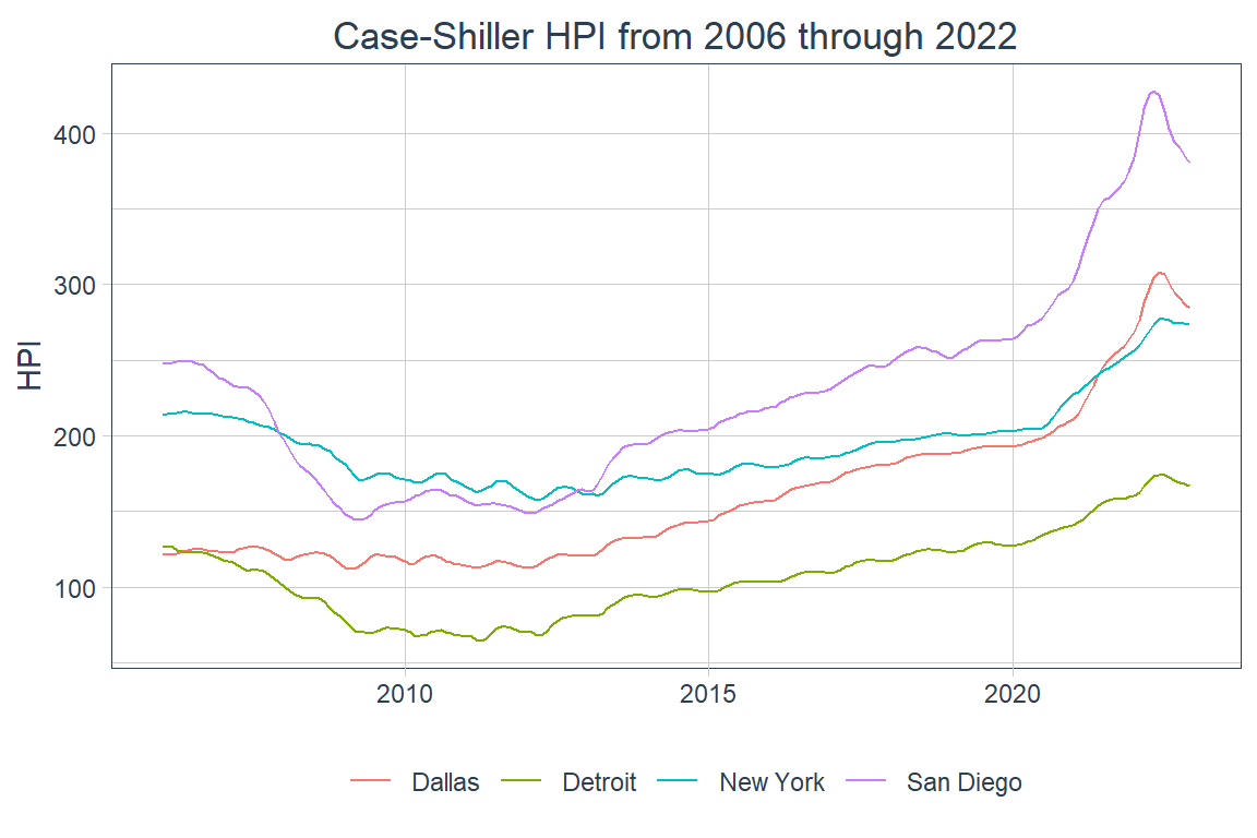
Here one can see that Dallas’s HPI did not drop as much during the Great Recession and has had a fast rise relative to those of the other cities ever since. It’s also pretty clear that NYC’s HPI has experienced a relatively mild increase over the years covered. There’s also more volatility between 2010 and 2015 in the HPIs for NYC, Dallas, and Detroit than in San Diego’s.
Time series analysis
The goal of this initial analysis is to find the parameters to use in an ARIMA model, which means that I’ll need to ensure my data are stationary. I’ll try to get there through the following operations and analyses.
Preparing the data
Before performing any analysis I’d like to add one column with a lagged first-difference and another with a lagged twelfth-difference. To accomplish this I’ll use the tk_augment_differences() from the timetk package. I’ll store this data set in a new variable called “hpi_series”. I chose these two lagged differences because the lagged first-difference generally any stationarity rooted in a trend and the lagged twelfth-difference should deal with seasonality as my data are monthly observations and I’m operating on the assumption that the housing market cycle is annual.
Below is a snippet of the data.
Code
| city | date | hpi | hpi_lag1_diff1 | hpi_lag1_diff12 |
|---|---|---|---|---|
| Dallas | 2006-01-01 | 121.9108 | NA | NA |
| Dallas | 2006-02-01 | 121.3285 | -0.58234 | NA |
| Dallas | 2006-03-01 | 121.5217 | 0.19324 | NA |
| Dallas | 2006-04-01 | 122.3996 | 0.87788 | NA |
| Dallas | 2006-05-01 | 123.2863 | 0.88666 | NA |
| Dallas | 2006-06-01 | 124.4985 | 1.21228 | NA |
| Dallas | 2006-07-01 | 125.3672 | 0.86869 | NA |
| Dallas | 2006-08-01 | 125.7007 | 0.33342 | NA |
| Dallas | 2006-09-01 | 125.1859 | -0.51474 | NA |
| Dallas | 2006-10-01 | 124.5813 | -0.60463 | NA |
| Dallas | 2006-11-01 | 123.8517 | -0.72958 | NA |
| Dallas | 2006-12-01 | 123.6697 | -0.18205 | NA |
| Dallas | 2007-01-01 | 122.6361 | -1.03360 | -161.2924 |
| Dallas | 2007-02-01 | 122.7292 | 0.09314 | 188.2084 |
| Dallas | 2007-03-01 | 123.1562 | 0.42699 | -251.1343 |
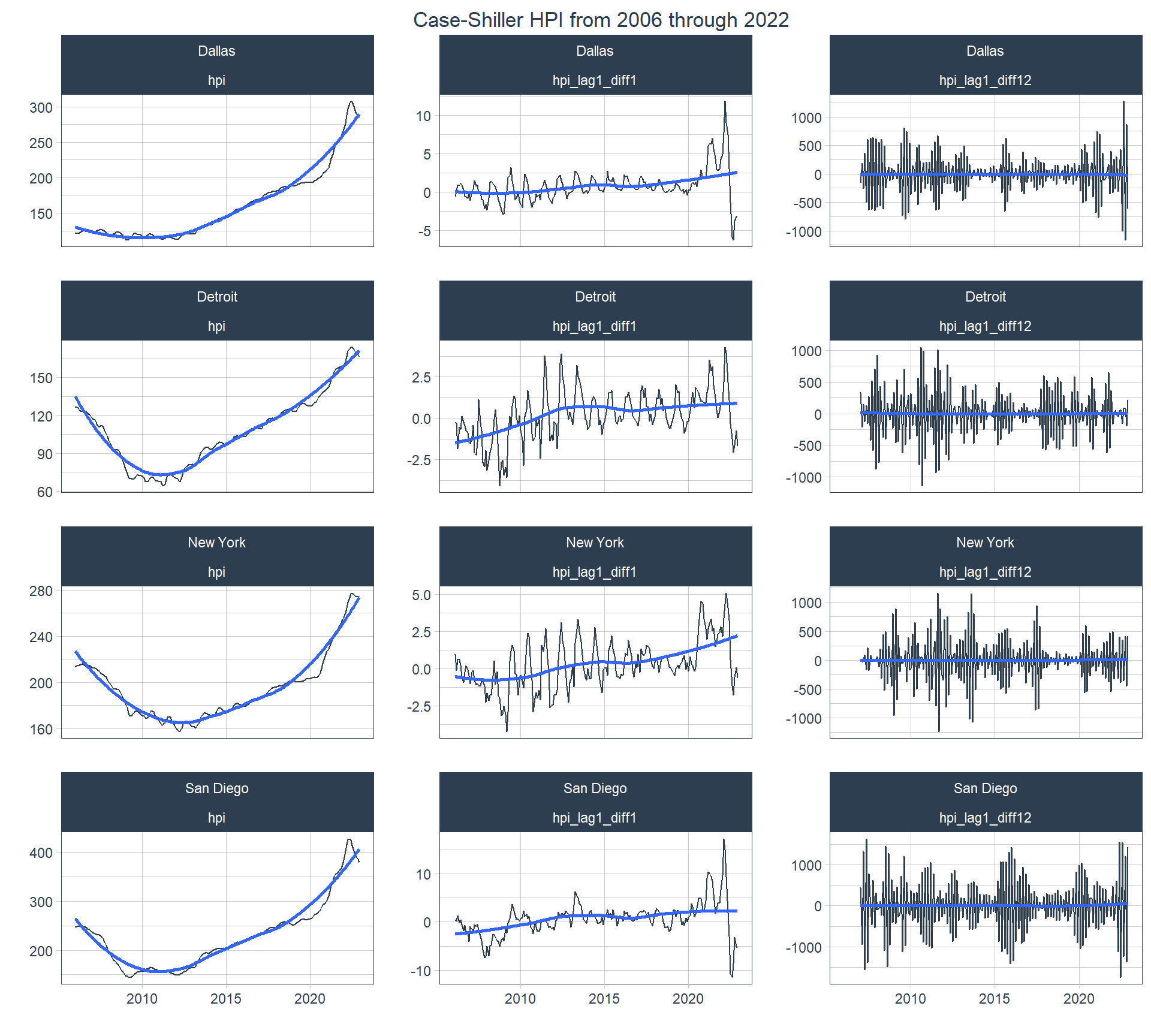
And now I can look at line plots of the three different series with the original on the left ; the lagged first-difference in the middle; and the lagged twelfth-difference on the right with a the cities in the different rows. From left to right the plots go from being highly regular (seasonal and trending) to being less regular in the middle (only seasonal) and highly irregular on the right. That irregularity is indicative of stationarity, which is what I want to see. This also provides a sneak peak into what the following analyses will give us.
Code
On might ask “why not use a lagged, log difference?” The below plot shows that using a lagged, log first- and twelfth-differenced series don’t change anything compared to the lagged first- and twelfth-differenced series except for generating data with much higher relative amplitude and possibly showing outliers. This might actually introduce heteroskedasticity, which I’d like to avoid.
Code
econ_data |>
  tk_augment_differences(
    .value = hpi,
    .lags = 1,
    .differences = c(1, 12),
    .log = TRUE
  ) |>
  pivot_longer(starts_with("hpi"), names_to = "series", values_to = "value") |>
  group_by(city, series) |>
  plot_time_series(
    date,
    value,
    .facet_ncol = 3,
    .title = "Case-Shiller HPI from 2006 through 2022",
    .interactive = FALSE
  ) +
  theme(plot.title = element_text(hjust = 0.5))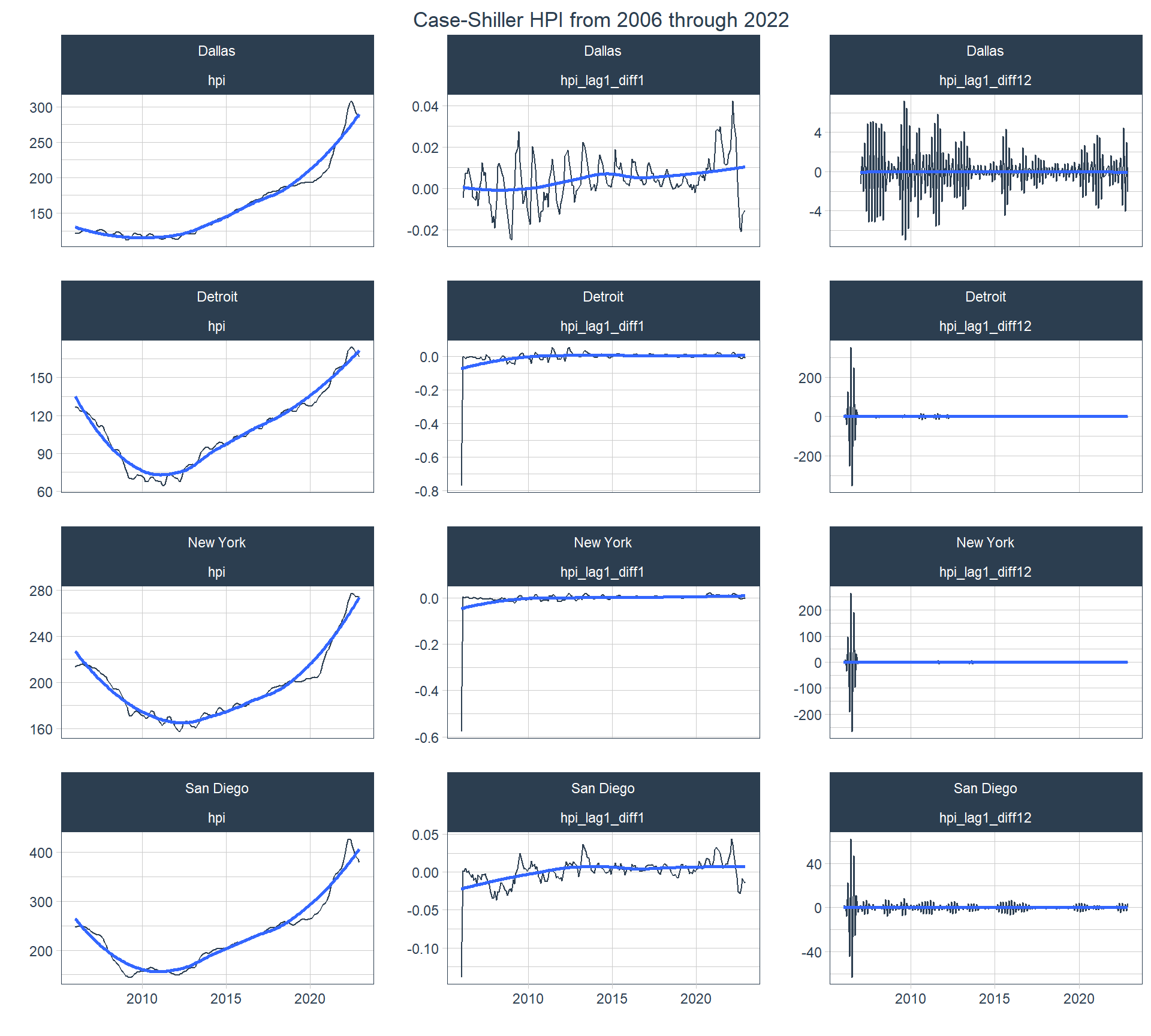
Time series decomposition
The following plot shows the Seasonal-Trend decomposition using Loess (STL), which is a common tool to determine how much of a time series’ movement is due to a trend versus that which is due to it’s seasonality. Again, here I’ll assume an annual seasonal cycle.
Code
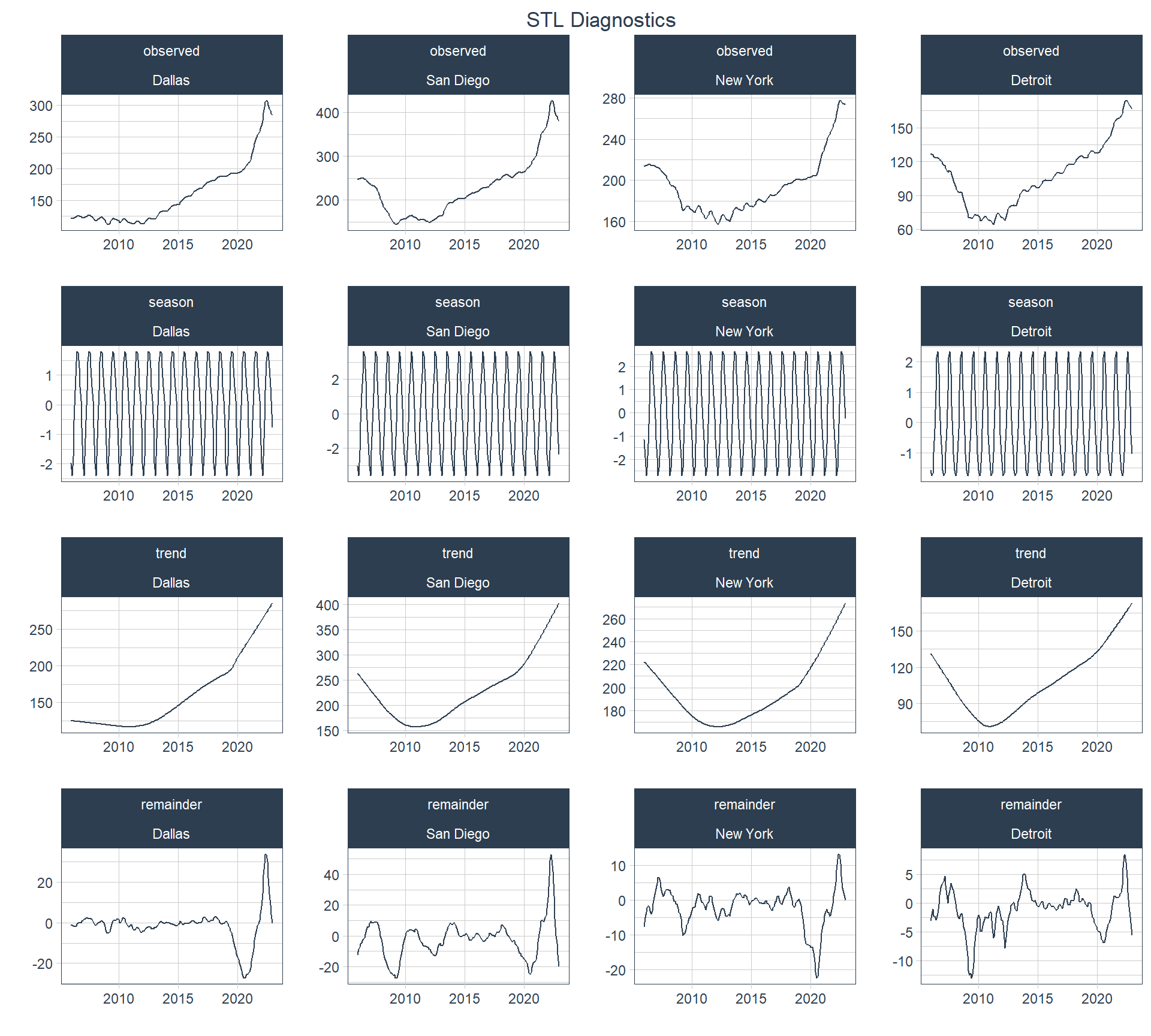
According to this plot most of the movement in the HPI is determined by the trend and very little by seasonality.
Augmented Dickey-Fuller Test
The Augmented Dickey-Fuller Test (ADF) is commonly run to evaluate whether a time series is stationary or not. The null hypothesis of the ADF is that the time series is non-stationary, so want to reject the null hypothesis to be able to assume the alternative, i.e., that the series is stationary. The following table shows that one can reject the null hypothesis for every city but San Diego with just a lagged first-difference, but with the lagged twelfth-difference all four series can be thought of as stationary.
Code
hpi_adf <- hpi_series |>
  pivot_longer(!c(city, date), names_to = "variable") |>
  group_by(city, variable) |>
  nest(data = c(date, value)) |>
  mutate(
    adf_test = map(
      data,
      \(x) drop_na(x, value) |>
        pull(value) |>
        tseries::adf.test() |>
        broom::tidy() |>
        select(statistic, p.value)
    )
  ) |>
  select(-data) |>
  unnest(adf_test) |>
  ungroup(variable)

hpi_adf |>
  group_by(city) |>
  group_nest() |>
  mutate(data_gt = map(data, make_adf_gt)) |>
  select(!data) |>
  pivot_wider(names_from = city, values_from = data_gt) |>
  gt() |>
gt_bold_head()| Dallas | Detroit | New York | San Diego | ||||||||||||
|---|---|---|---|---|---|---|---|---|---|---|---|---|---|---|---|
|
|
|
|
ACF / PACF plots
The Autocorrelation Function (ACF) calculates the correlation of a value, e.g., the most recent value of the HPI, with previous values in the same series. Knowing this is very useful for determining how many Moving Average (the “MA” in ARIMA) lags to use in an ARIMA mode. The Partial Autocorrelation Function (PACF) calculates the correlation of a value with previous values in the same series after accounting for intervening correlations. This is useful to help us determine how many lags to use for the Autoregressive (the “AR” in ARIMA) part of an ARIMA model. Below are the ACF and PACF plots for the HPI series (no lagged differences) for all four cities. The timetk::plot_acf_diagnostics() function plots ACF on top and PACF on bottom, which is conventional. Values outside of the red, dashed lines indicate statistically significant correlations.
Code
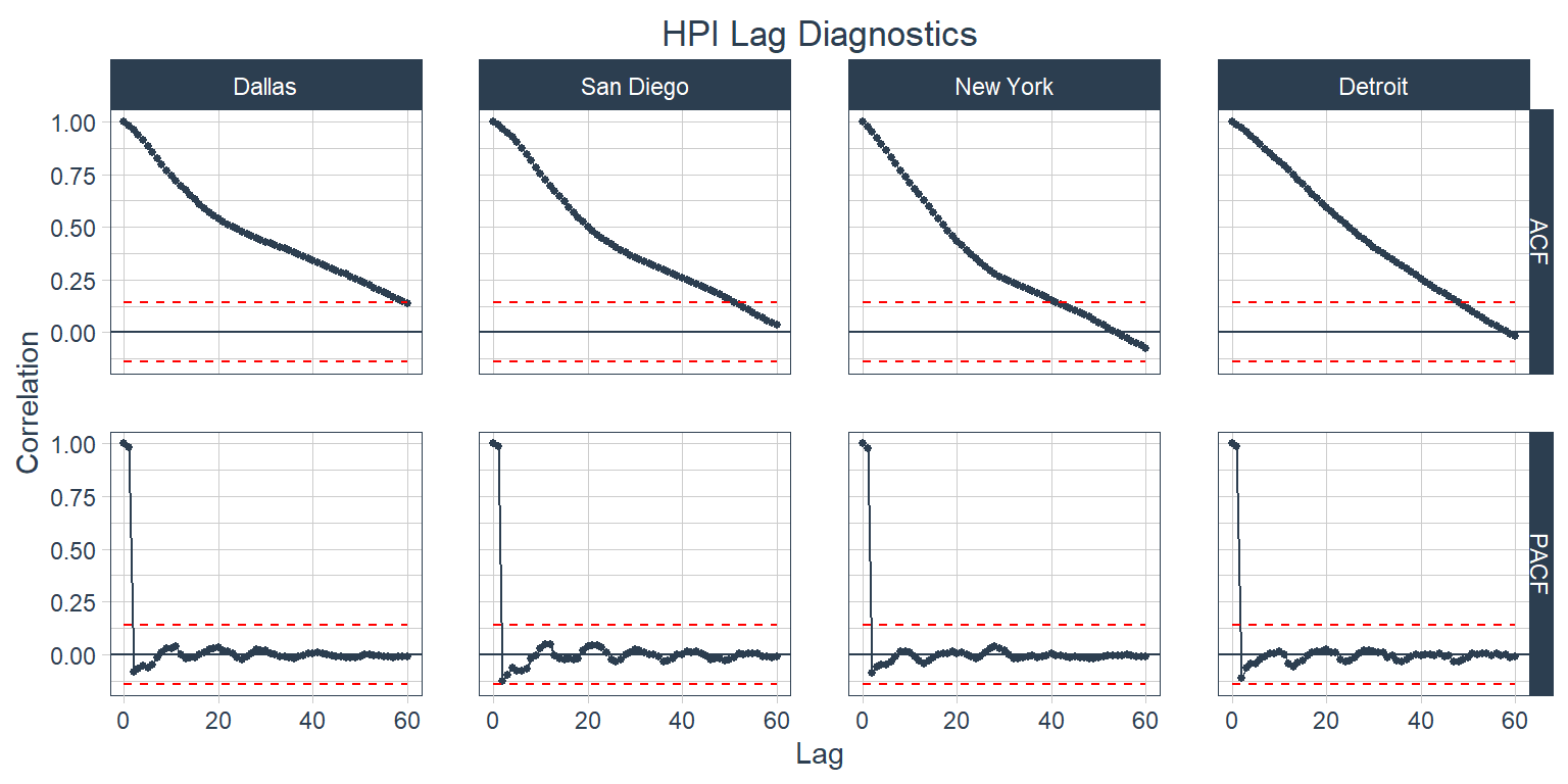
It’s clear from the ACF plot that the trend is causing a lot of the autocorrelation in each city. Next is the same plot, but for the first-differenced values.
Code
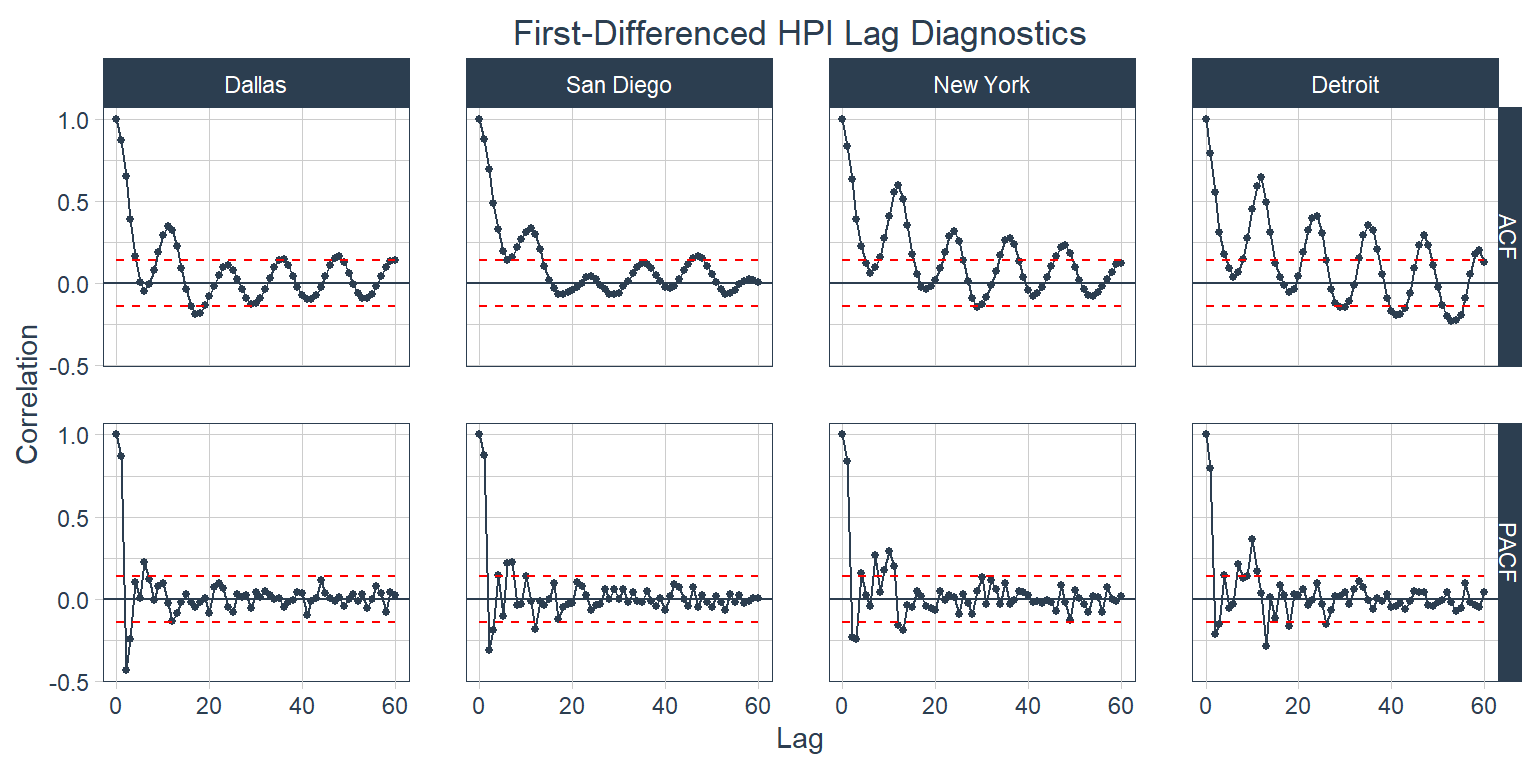
The trend’s influence is significantly decreased here, but there are still some strong seasonal patterns in the data. Below is a look at the twelfth-differenced series.
Code
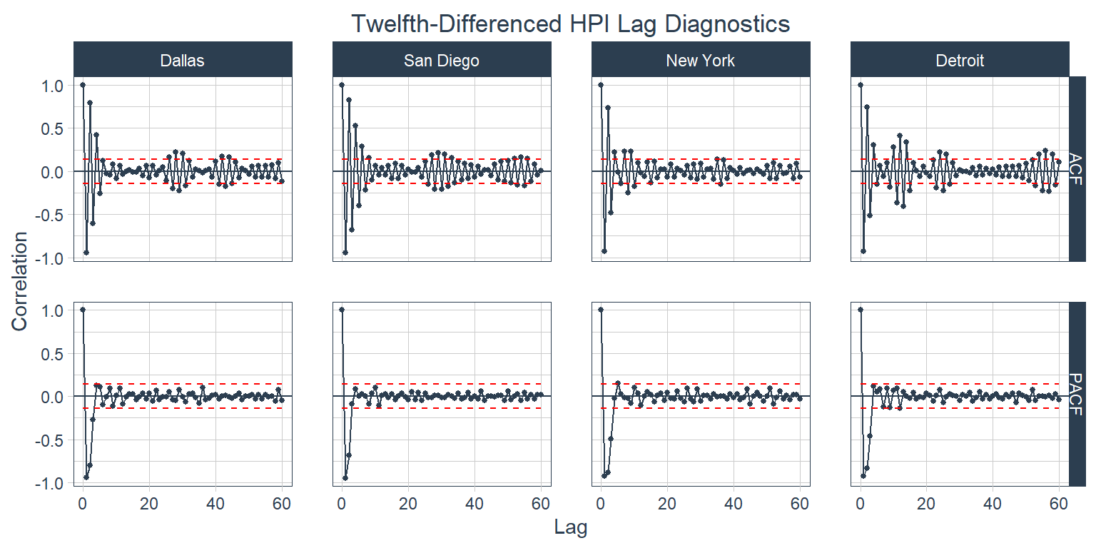
Looking at this plot over 36 months it still appears that there is a small seasonal effect in Dallas, San Diego, and Detroit with Detroit’s possibly being a shorter season. Considering the infinite number of things that could affect one of these data series one could look at hundreds of plots like this with different combinations of lags and differences for any one series and never find a perfect one. This plot is pretty good. From this plot it looks like I’m going to us an AR(3) model. San Diego’s PACF suggests that I should use two for that city, but I’m looking for one value for all four cities. The MA component is a little more challenging. It looks like I would use MA lags of 5 or 6 for Dallas, 8 for San Diego, 4 for NYC, and 4 or 5 for Detroit. I’m going to use MA(5) for my ARIMA.
Seasonality
It’s been pretty clear up to this point that seasonality is an important consideration with this data series and it’s something that I will expect to handle in the modeling portion of the analysis in a later post. If I wanted to handle seasonality in a conventional model I might run a SARIMA model, but I’m going to keep this part simple and only run ARIMA knowing that I’m partially ignoring the seasonality and only dealing with it by differencing. With that said, I’ll show two more plots here to demonstrate the timetk::plot_seasonal_diagnostics() . The first plot shows seasonal diagnostics for the unadjusted series and the second one for the twelfth-differenced series.
Code
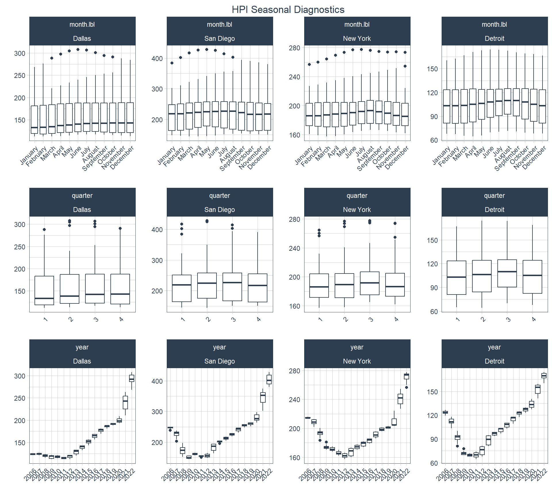
This plot shows a clear pattern of HPI values being lowest in the first quarter across all four cities, highest in the second and third quarters for San Diego, and highest in the quarter for New York and December. From this data it seems that the peak in Dallas is December. This seasonality can obscure the findings of an ARIMA model.
Code
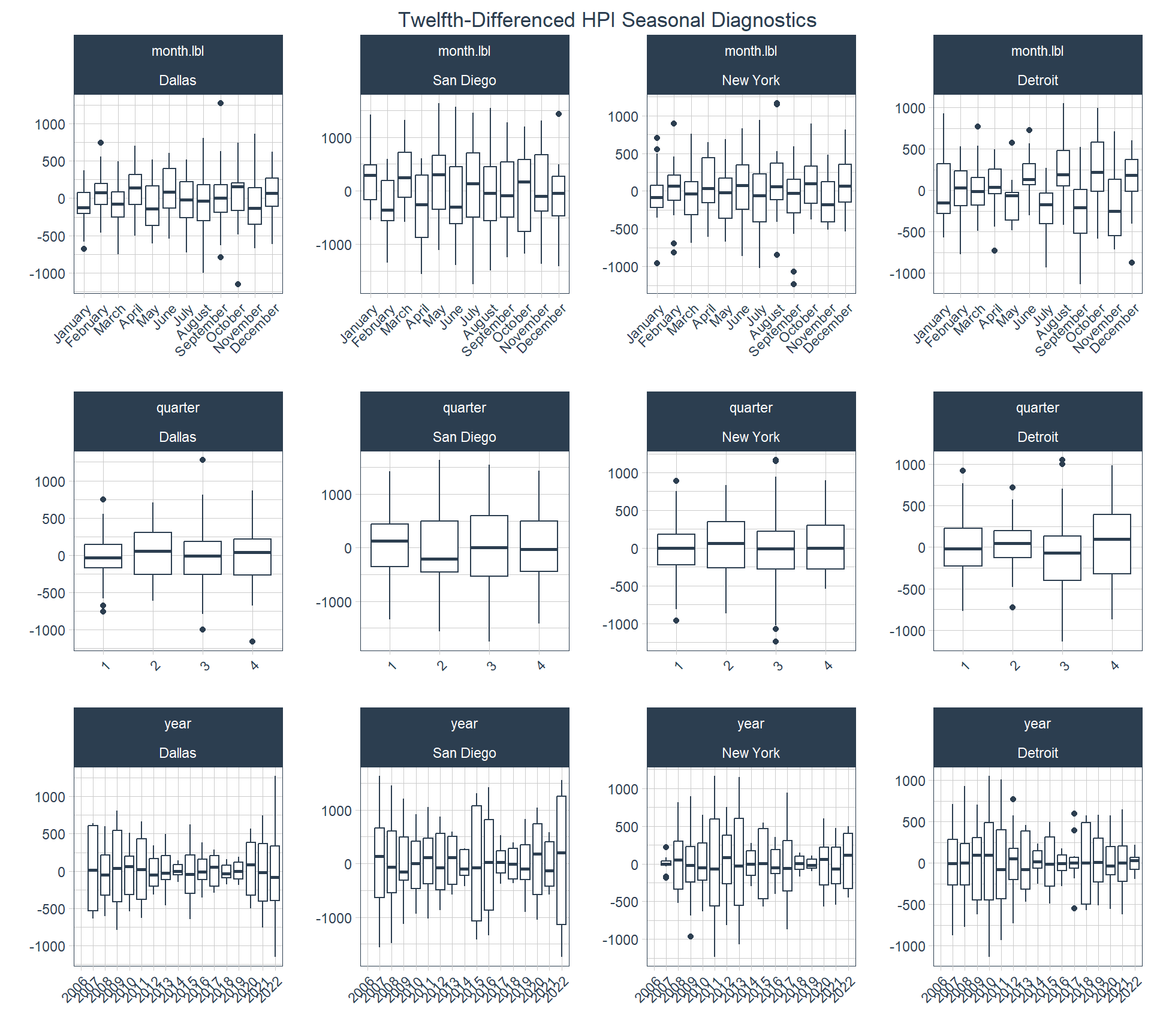
In this plot the patterns are generally gone across the quarterly plots. Even the trend is mostly gone from the annual plot.
In the next post I’ll use the AR and MA values from this post to run ARIMA models for all four cities using a global modeling process and an iterative modeling process with modeltime.