Forecasting with {modeltime} - Part V

Selecting the best model for each city

This is the final (planned) post for this series on the modeltime (Dancho 2023) package I will identify the best model to forecast the Case-Shiller Home Price Index using an iterative modeling process. The models to work with will be the 11 models that I identified through the global modeling process in Forecasting with {modeltime} - Part IV. Additionally I’ll be using parallel (2023) for parallel processing, tidymodels (Kuhn and Wickham 2020) for a modeling framework, tidyverse (Wickham et al. 2019) for data wrangling and visualization, and gt (Iannone et al. 2024) for table output.

library(tidyverse)
library(timetk)
library(modeltime)
library(tidymodels)
library(parallel)
library(gt)
conflicted::conflict_prefer("filter", "dplyr")
conflicted::conflict_prefer("lag", "dplyr")
tidymodels_prefer()

Below is a look at the names of the model specifications from the last post.

part4_mods |> gt() |> gt_bold_head()

.model_desc
BASE_REC_ETS_DEFAULT
BASE_REC_ARIMA_DEFAULT
BASE_REC_ARIMA_SPEC2
BASE_REC_ETS_SPEC14
BASE_REC_ETS_SPEC6
DEMOG_REC_ARIMA_SPEC1
DEMOG_REC_ARIMA_SPEC3
NNET_REC_NNET_SPEC22
NNET_REC_NNET_SPEC9
NNET_REC_NNET_SPEC12
BASE_REC_STLM_SPEC3

And this is what the workflowset object looked like.

hpi_global_wfset

# A workflow set/tibble: 90 × 4
   wflow_id               info             option    result    
   <chr>                  <list>           <list>    <list>    
 1 base_rec_arima_default <tibble [1 × 4]> <opts[0]> <list [0]>
 2 base_rec_arima_spec1   <tibble [1 × 4]> <opts[0]> <list [0]>
 3 base_rec_arima_spec2   <tibble [1 × 4]> <opts[0]> <list [0]>
 4 base_rec_arima_spec3   <tibble [1 × 4]> <opts[0]> <list [0]>
 5 base_rec_arima_spec4   <tibble [1 × 4]> <opts[0]> <list [0]>
 6 econ_rec_arima_default <tibble [1 × 4]> <opts[0]> <list [0]>
 7 econ_rec_arima_spec1   <tibble [1 × 4]> <opts[0]> <list [0]>
 8 econ_rec_arima_spec2   <tibble [1 × 4]> <opts[0]> <list [0]>
 9 econ_rec_arima_spec3   <tibble [1 × 4]> <opts[0]> <list [0]>
10 econ_rec_arima_spec4   <tibble [1 × 4]> <opts[0]> <list [0]>
# ℹ 80 more rows

Filtering workflows

I’ll first filter the set of workflows to the 11 that I want to keep.

mod_ids <- str_to_lower(part4_mods$.model_desc)

hpi_global_wfset <- hpi_global_wfset |>
  filter(wflow_id %in% mod_ids)

These are all of the necessary workflows including recipes and model specifications.

Splitting the data

Next up is creating the data split object. This is a different set of functions than what I used to split the data for the global modeling process. In this workflow the future dates get added for each city up front.

econ_splits <- econ_data |>
  extend_timeseries(
    .id_var = city,
    .date_var = date,
    .length_future = 12
  ) |>
  nest_timeseries(
    .id_var = city,
    .length_future = 12,
    .length_actual = 17 * 12
  ) |>
  split_nested_timeseries(.length_test = 24)

econ_splits

# A tibble: 4 × 4
  city      .actual_data        .future_data       .splits         
  <chr>     <list>              <list>             <list>          
1 Dallas    <tibble [204 × 15]> <tibble [12 × 15]> <split [180|24]>
2 Detroit   <tibble [204 × 15]> <tibble [12 × 15]> <split [180|24]>
3 New York  <tibble [204 × 15]> <tibble [12 × 15]> <split [180|24]>
4 San Diego <tibble [204 × 15]> <tibble [12 × 15]> <split [180|24]>

With these two objects prepared I can now fit the models iteratively for each city.

Fit models

I’ll first prepare a parallel processing cluster and set a random seed for each node then fit the models.

Note

modeltime_nested_fit() requires that models be specified individually rather than as a workflowset object.

cl <- makePSOCKcluster(nrow(part4_mods))
doParallel::registerDoParallel(cl)
invisible(
  clusterCall(cl, function(x) .libPaths(x), .libPaths())
)
print(cl)
invisible(clusterEvalQ(cl, set.seed(500)))

hpi_wflowset <- modeltime_nested_fit(
  econ_splits,
  hpi_global_wfset |> extract_workflow(mod_ids[1]),
  hpi_global_wfset |> extract_workflow(mod_ids[2]),
  hpi_global_wfset |> extract_workflow(mod_ids[3]),
  hpi_global_wfset |> extract_workflow(mod_ids[4]),
  hpi_global_wfset |> extract_workflow(mod_ids[5]),
  hpi_global_wfset |> extract_workflow(mod_ids[6]),
  hpi_global_wfset |> extract_workflow(mod_ids[7]),
  hpi_global_wfset |> extract_workflow(mod_ids[8]),
  hpi_global_wfset |> extract_workflow(mod_ids[9]),
  hpi_global_wfset |> extract_workflow(mod_ids[10]),
  hpi_global_wfset |> extract_workflow(mod_ids[11]),
  control = control_nested_fit(verbose = TRUE, allow_par = TRUE)
)

stopCluster(cl)
rm(cl)

hpi_wflowset |> as_tibble()

# A tibble: 4 × 5
  city      .actual_data        .future_data .splits          .modeltime_tables
  <chr>     <list>              <list>       <list>           <list>           
1 Dallas    <tibble [204 × 15]> <tibble>     <split [180|24]> <mdl_tm_t>       
2 Detroit   <tibble [204 × 15]> <tibble>     <split [180|24]> <mdl_tm_t>       
3 New York  <tibble [204 × 15]> <tibble>     <split [180|24]> <mdl_tm_t>       
4 San Diego <tibble [204 × 15]> <tibble>     <split [180|24]> <mdl_tm_t>       

Notice that this object is grouped by city whereas the corresponding object for the global modeling process is listed by model. This happens because modeltime_nested_fit() calls a split object that has the data grouped by ID already. All of the functions in the modeltime Nested Forecasting workflow geared toward doing things at the level of the ID variable, which is “city” in this case. Each row contains a mdl_time_tbl object in the “.modeltime_tables” column for each row which has one row for each model that was fit to the data of the ID in that row. This mdl_time_tbl object contains calibration data, which gets created during the iterative modeling process. Below is an example.

hpi_wflowset |> slice(1) |> pluck(".modeltime_tables", 1)

# Modeltime Table
# A tibble: 11 × 5
   .model_id .model       .model_desc           .type .calibration_data
       <int> <named list> <chr>                 <chr> <list>           
 1         1 <workflow>   ETSAADN               Test  <tibble [24 × 4]>
 2         2 <workflow>   ARIMA                 Test  <tibble [24 × 4]>
 3         3 <workflow>   ARIMA                 Test  <tibble [24 × 4]>
 4         4 <workflow>   ETSAADA               Test  <tibble [24 × 4]>
 5         5 <workflow>   ETSAADA               Test  <tibble [24 × 4]>
 6         6 <workflow>   REGRESSION            Test  <tibble [24 × 4]>
 7         7 <workflow>   REGRESSION            Test  <tibble [24 × 4]>
 8         8 <NULL>       NULL                  <NA>  <lgl [1]>        
 9         9 <NULL>       NULL                  <NA>  <lgl [1]>        
10        10 <NULL>       NULL                  <NA>  <lgl [1]>        
11        11 <workflow>   SEASONAL DECOMP ARIMA Test  <tibble [24 × 4]>

Selecting the best models

{modeltime} has the modeltime_nested_select_best() for selecting the best model for each ID in a nested model table. It requires the specification of a metric for determining which model is “best”. As before, I’ll use the Scaled Mean Average Percent Error (SMAPE).

hpi_best <- hpi_wflowset |>
  modeltime_nested_select_best(
    metric = "smape",
    minimize = TRUE,
    filter_test_forecasts = TRUE
  )

hpi_best

# Nested Modeltime Table
  # A tibble: 4 × 5
  city      .actual_data        .future_data .splits          .modeltime_tables 
  <chr>     <list>              <list>       <list>           <list>            
1 Dallas    <tibble [204 × 15]> <tibble>     <split [180|24]> <mdl_tm_t [1 × 5]>
2 Detroit   <tibble [204 × 15]> <tibble>     <split [180|24]> <mdl_tm_t [1 × 5]>
3 New York  <tibble [204 × 15]> <tibble>     <split [180|24]> <mdl_tm_t [1 × 5]>
4 San Diego <tibble [204 × 15]> <tibble>     <split [180|24]> <mdl_tm_t [1 × 5]>

Notice that after selecting the best model it’s only the “.modeltime_tables” column that changes. It now contains a table with one single row corresponding to the model that yielded the best value of the selected metric.

View accuracy best models

One gets the accuracy from a nested modeltime table by using extract_nested_test_accuracy() . Interestingly, this function shows the accuracy of all models even if it’s run with the table of the “best” models. So below I’ll use group_by() to get the accuracy for the best model for each city.

hpi_wflowset |>
  extract_nested_test_accuracy() |>
  group_by(city) |>
  slice_min(smape, n = 1) |>
  ungroup() |>
  table_modeltime_accuracy(.interactive = FALSE) |>
  gt_bold_head()

Accuracy Table
city	.model_id	.model_desc	.type	mae	mape	mase	smape	rmse	rsq
Dallas	11	SEASONAL DECOMP ARIMA	Test	39.49	14.11	7.54	15.46	44.89	0.86
Detroit	11	SEASONAL DECOMP ARIMA	Test	4.16	2.56	2.37	2.59	4.80	0.86
New York	11	SEASONAL DECOMP ARIMA	Test	9.12	3.50	3.84	3.58	10.70	0.90
San Diego	6	REGRESSION	Test	30.77	8.19	4.36	7.75	35.89	0.29

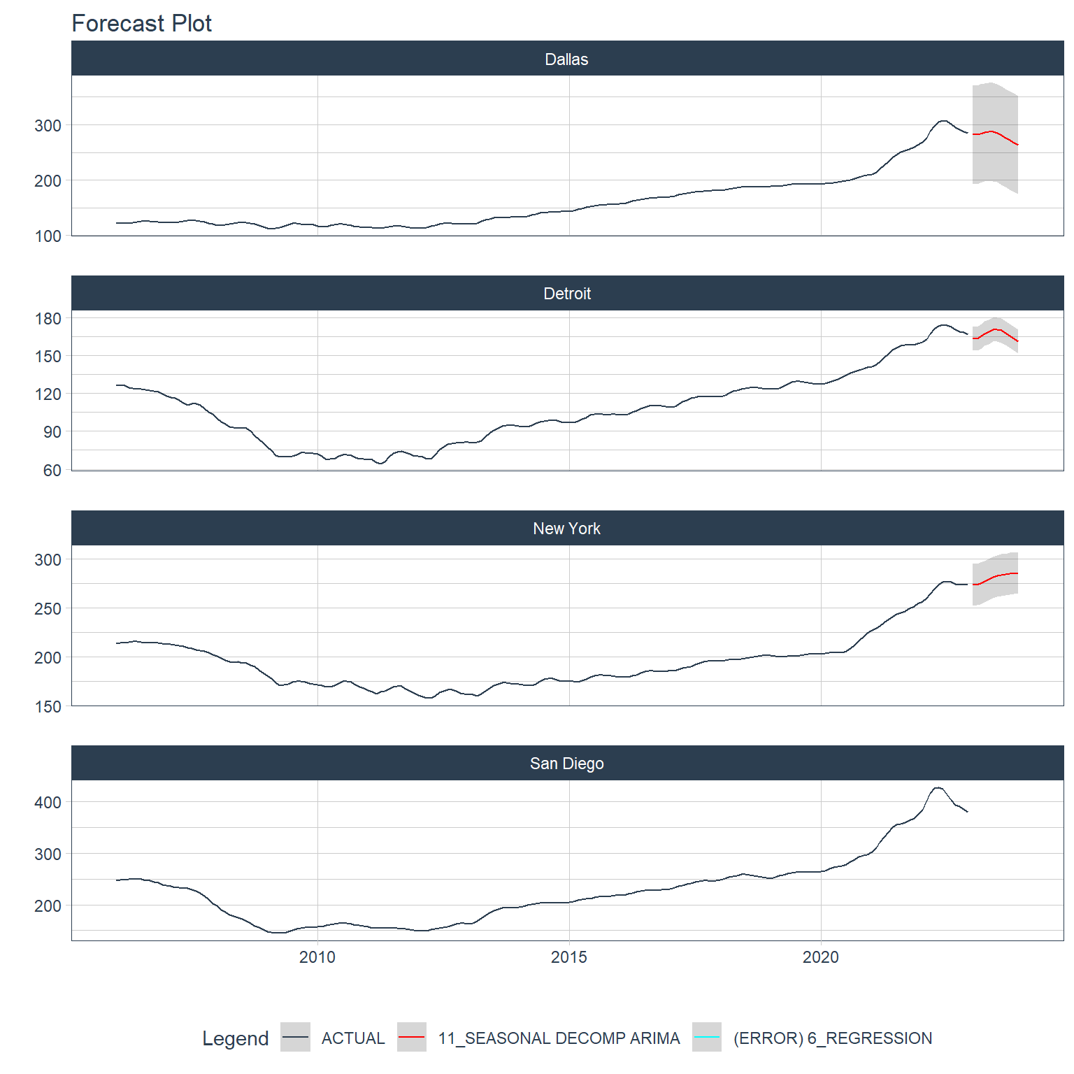
Next are the forecasts against the test data.

fcst_pal <- c(
  "#2c3e50", "#FF0000", "#00FFFF", "#FFFF00", "#0000FF", "#00FF00",
  "#FF00FF", "#FF8000", "#0080FF", "#80FF00", "#8000FF", "#00FF80",
  "#FF0080"
)

hpi_best |>
  extract_nested_test_forecast() |>
  group_by(city) |>
  plot_modeltime_forecast(.interactive = FALSE) +
  scale_color_manual(values = fcst_pal)

1

Create a color palette for plotting.

Figure 1

For Dallas, Detroit, and New York the 11th model in the original workflow which is a Seasonal Decomposition ARIMA model and for San Diego it’s the 6th model which is just called “REGRESSION”. I’ll show the table of model names here here with a “model_num” column indicating model number.

part4_mods |>
  mutate(model_num = row_number()) |>
  gt() |>
  gt_bold_head()

.model_desc	model_num
BASE_REC_ETS_DEFAULT	1
BASE_REC_ARIMA_DEFAULT	2
BASE_REC_ARIMA_SPEC2	3
BASE_REC_ETS_SPEC14	4
BASE_REC_ETS_SPEC6	5
DEMOG_REC_ARIMA_SPEC1	6
DEMOG_REC_ARIMA_SPEC3	7
NNET_REC_NNET_SPEC22	8
NNET_REC_NNET_SPEC9	9
NNET_REC_NNET_SPEC12	10
BASE_REC_STLM_SPEC3	11

We can see that the 11th model is an STLM model and the 6th model is the first ARIMA specification with the “DEMOG” recipe (this is the one that included economic and demographic covariates).

The plot for San Diego does not include a margin of error and it’s listed as having an error in the legend. This is something that can be traced to the calibration. First I’ll extract the “.modeltime_tables”.

hpi_wflowset |>
  filter(city %in% "San Diego") |>
  pluck(".modeltime_tables", 1)

# Modeltime Table
# A tibble: 11 × 5
   .model_id .model       .model_desc           .type .calibration_data
       <int> <named list> <chr>                 <chr> <list>           
 1         1 <workflow>   ETSAADN               Test  <tibble [24 × 4]>
 2         2 <workflow>   ARIMA                 Test  <tibble [24 × 4]>
 3         3 <workflow>   ARIMA                 Test  <tibble [24 × 4]>
 4         4 <workflow>   ETSAADA               Test  <tibble [24 × 4]>
 5         5 <workflow>   ETSAADA               Test  <tibble [24 × 4]>
 6         6 <workflow>   REGRESSION            Test  <tibble [24 × 4]>
 7         7 <workflow>   REGRESSION            Test  <tibble [24 × 4]>
 8         8 <NULL>       NULL                  <NA>  <lgl [1]>        
 9         9 <NULL>       NULL                  <NA>  <lgl [1]>        
10        10 <NULL>       NULL                  <NA>  <lgl [1]>        
11        11 <workflow>   SEASONAL DECOMP ARIMA Test  <tibble [24 × 4]>

I can see that the 6th model does contain calibration data, so this isn’t the problem. Now I’ll extract the calibration data just for this model to see what’s going on.

hpi_wflowset |>
  filter(city %in% "San Diego") |>
  pluck(".modeltime_tables", 1) |>
  filter(.model_id == 6) |>
  pluck(".calibration_data", 1)

# A tibble: 24 × 4
   date       .actual .prediction .residuals
   <date>       <dbl>       <dbl>      <dbl>
 1 2021-01-01    302.         NA        NA  
 2 2021-02-01    311.         NA        NA  
 3 2021-03-01    321.         NA        NA  
 4 2021-04-01    332.         NA        NA  
 5 2021-05-01    341.         NA        NA  
 6 2021-06-01    350.         NA        NA  
 7 2021-07-01    355.        409.      -53.6
 8 2021-08-01    357.        410.      -53.2
 9 2021-09-01    360.        412.      -51.6
10 2021-10-01    364.        413.      -48.8
# ℹ 14 more rows

Gaaaahhhh! It’s the missing data created by the lags in the recipe for this model. It might be interesting to run this model again without those lags, but I’ll be happy just to know why there is no margin of error for this one. Interestingly, though, it looks like the STLM did a pretty good job with Detroit and New York.

Now it’s on to forecasting the future.

Forecasting future HPI

The first step in forecasting is re-fitting the models to the full data set including the test portion. I’ll do this with modeltime_nested_refit() . I’ll immediately use that refit object to plot the forecasts.

hpi_refit <- hpi_best |>
  modeltime_nested_refit(control = control_nested_refit(verbose = FALSE))

hpi_refit |>
  extract_nested_future_forecast() |>
  group_by(city) |>
  plot_modeltime_forecast(.interactive = FALSE) +
  scale_color_manual(values = fcst_pal)

It looks like the missing values due to the lags prevented the ARIMA from generating forecasts, but the other forecasts look quite believable and much better than the forecasts made by the global process.

Comparing forecasts to what really happened

I used data that ended in December 2022 because that’s the most recent data I had for some demographic variables. This isn’t a problem for the STLM since this model doesn’t rely on demographic covariates, but there is HPI data through September of 2023, and the forecasts go through December of 2023. So, here I’ll just get the HPI data for 2023 for Dallas, Detroit, and New York.

case_shiller_ids <- fredr::fredr_series_search_text("Case-Shiller") |>
  filter(
    str_detect(
      title,
      "TX-Dallas|NY-New York|MI-Detroit Home Price Index"
    ),
    seasonal_adjustment_short %in% "NSA",
    frequency %in% "Monthly"
  ) |>
  mutate(city = str_extract(title, "New York|Dallas|San Diego|Detroit")) |>
  select(city, id)

# Get Case Shiller data for 2023
hpi_data <- case_shiller_ids |>
  mutate(
    data = map(
      id,
      \(x) fredr::fredr(
        series_id = x,
        observation_start = ymd("2020-01-01"),
        observation_end = ymd("2023-12-31"),
        frequency = "m"
      )
    )
  ) |>
  select(-id) |>
  unnest(data) |>
  select(city, date, hpi = value)

hpi_data |>
  pivot_wider(names_from = city, values_from = hpi) |>
  filter(year(date) == 2023) |>
  gt() |>
  gt_bold_head()

date	Dallas	New York	Detroit
2023-01-01	281.7092	272.8493	165.3712
2023-02-01	281.6864	271.9243	165.0817
2023-03-01	284.7053	274.9276	168.7419
2023-04-01	288.6548	278.5348	172.7052
2023-05-01	293.1761	283.2171	176.2015
2023-06-01	295.2387	286.5359	177.9996
2023-07-01	296.1252	289.0024	179.2959
2023-08-01	295.6140	290.5704	180.7211
2023-09-01	295.2280	292.3354	181.9622
2023-10-01	294.2782	293.4502	182.6364
2023-11-01	292.4071	294.2285	181.8668

Now I can make a table of accuracy statistics for these series.

hpi_data |>
  left_join(
    hpi_refit |>
      filter(!city %in% "San Diego") |>
      extract_nested_future_forecast() |>
      filter(.key %in% "prediction") |>
      unite("model_name", .model_id, .model_desc) |>
      select(!.key),
    by = c("city", "date" = ".index")
  ) |>
  group_nest(city) |>
  mutate(
    smape = map_dbl(
      data,
      \(x) smape(x, hpi, .value) |> pull(.estimate)
    ),
    rmse = map_dbl(
      data,
      \(x) rmse(x, hpi, .value) |> pull(.estimate)
    ),
    rsq = map_dbl(
      data,
      \(x) rsq(x, hpi, .value) |> pull(.estimate)
    )
  ) |>
  select(-data) |>
  ungroup() |>
  gt() |>
  gt_bold_head()

city	smape	rmse	rsq
Dallas	3.522232	13.336181	0.0272001
Detroit	5.161485	10.526957	0.2394261
New York	1.658322	5.643017	0.9973690

These are some pretty low (good) values of SMAPE. Let’s see what these look like in plots.

hpi_data |>
  mutate(model_name = "ACTUAL") |>
  rename(.value = hpi) |>
  bind_rows(
    hpi_refit |>
      extract_nested_future_forecast() |>
      filter(.key %in% "prediction", !city %in% "San Diego") |>
      unite("model_name", .model_id, .model_desc) |>
      select(!.key) |>
      rename(date = .index)
  ) |>
  mutate(
    model_name = fct_relevel(model_name, "ACTUAL"),
    lwidth = if_else(model_name %in% "ACTUAL", 1, 2)
  ) |>
  ggplot(aes(x = date, group = model_name, color = model_name)) +
  geom_line(aes(y = .value, linewidth = lwidth)) +
  geom_ribbon(aes(ymin = .conf_lo, ymax = .conf_hi), alpha = 0.2, color = NA) +
  scale_color_manual(values = fcst_pal) +
  scale_y_continuous(expand = c(0.5, 0.5)) +
  scale_linewidth(range = c(0.5, 1)) +
  facet_wrap(~ city, scales = "free_y", ncol = 1) +
  labs(
    color = NULL,
    x = NULL,
    y = NULL,
    title = "Forecasts vs. Actual Data"
  ) +
  guides(linewidth = "none") +
  theme_timetk +
  theme(plot.title = element_text(hjust = 0.5))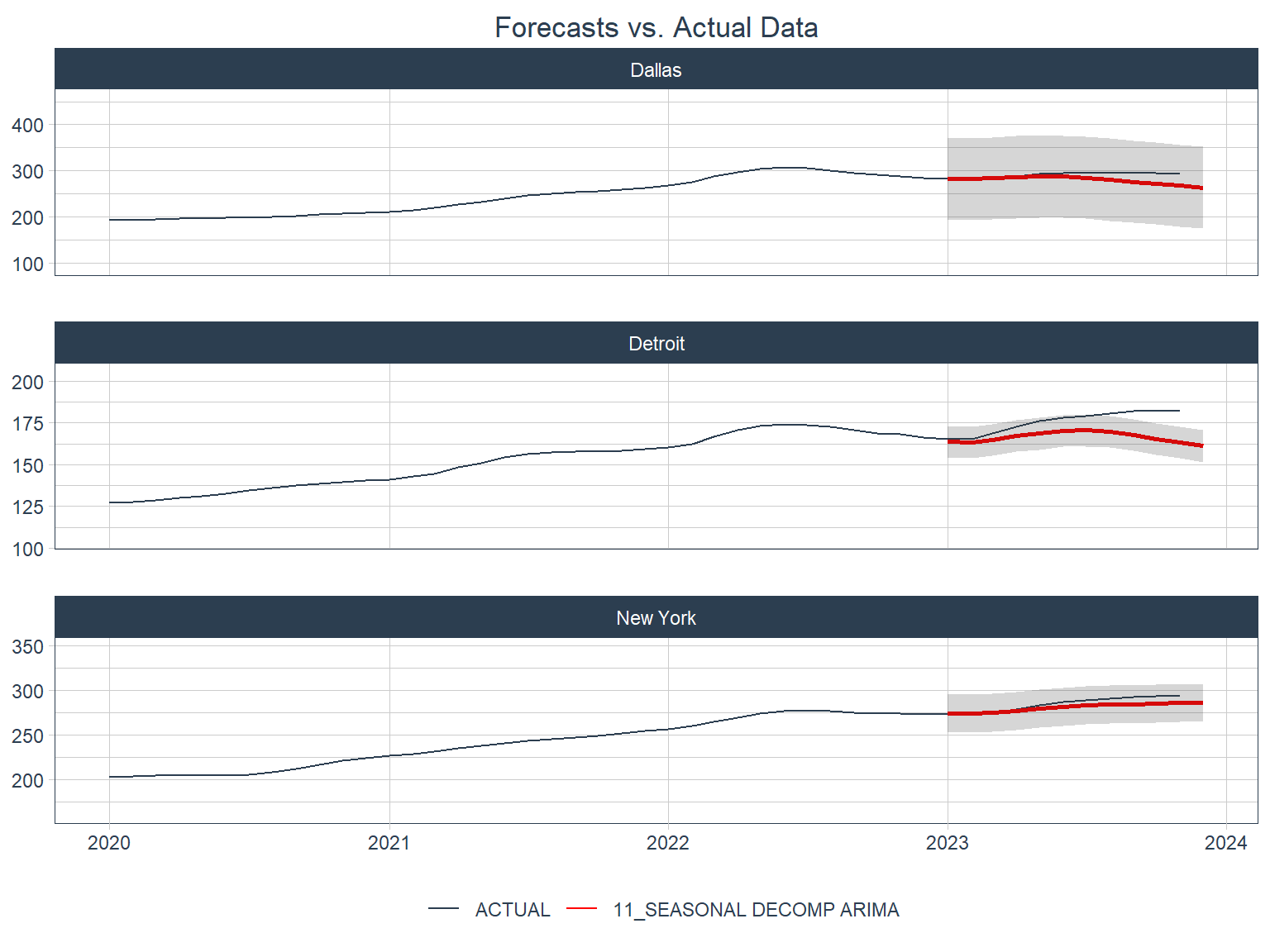

Not too bad! All three forecasts look like they were very close in the first few months of the forecast period, but started to underestimate later on.

This ends the series of planned posts on using modeltime with R. All in all this is a great package with all sorts of goodies for forecasting time series.

References

Dancho, Matt. 2023. “Modeltime: The Tidymodels Extension for Time Series Modeling.” https://CRAN.R-project.org/package=modeltime.

Iannone, Richard, Joe Cheng, Barret Schloerke, Ellis Hughes, Alexandra Lauer, and JooYoung Seo. 2024. “Gt: Easily Create Presentation-Ready Display Tables.” https://CRAN.R-project.org/package=gt.

Kuhn, Max, and Hadley Wickham. 2020. “Tidymodels: A Collection of Packages for Modeling and Machine Learning Using Tidyverse Principles.” https://www.tidymodels.org.

R Core Team. 2023. “R: A Language and Environment for Statistical Computing.” https://www.R-project.org/.

Wickham, Hadley, Mara Averick, Jennifer Bryan, Winston Chang, Lucy D’Agostino McGowan, Romain François, Garrett Grolemund, et al. 2019. “Welcome to the Tidyverse” 4: 1686. https://doi.org/10.21105/joss.01686.